---------------------------------------------------------------------------
ValueError                                Traceback (most recent call last)
Cell In[1], line 9
      7 import numpy as np
      8 from scipy import stats
----> 9 import statsmodels.api as sm
     10 import warnings
     11 warnings.filterwarnings("ignore")

File /opt/miniconda3/lib/python3.12/site-packages/statsmodels/api.py:125
    114 from .genmod import api as genmod
    115 from .genmod.api import (
    116     GEE,
    117     GLM,
   (...)
    123     families,
    124 )
--> 125 from .graphics import api as graphics
    126 from .graphics.gofplots import ProbPlot, qqline, qqplot, qqplot_2samples
    127 from .imputation.bayes_mi import MI, BayesGaussMI

File /opt/miniconda3/lib/python3.12/site-packages/statsmodels/graphics/api.py:9
      7 from .gofplots import qqplot
      8 from .plottools import rainbow
----> 9 from .regressionplots import (
     10     abline_plot,
     11     influence_plot,
     12     plot_ccpr,
     13     plot_ccpr_grid,
     14     plot_fit,
     15     plot_leverage_resid2,
     16     plot_partregress,
     17     plot_partregress_grid,
     18     plot_regress_exog,
     19 )
     21 __all__ = [
     22     "abline_plot",
     23     "beanplot",
   (...)
     42     "violinplot",
     43 ]

File /opt/miniconda3/lib/python3.12/site-packages/statsmodels/graphics/regressionplots.py:23
     21 from statsmodels.genmod.generalized_linear_model import GLM
     22 from statsmodels.graphics import utils
---> 23 from statsmodels.nonparametric.smoothers_lowess import lowess
     24 from statsmodels.regression.linear_model import GLS, OLS, WLS
     25 from statsmodels.sandbox.regression.predstd import wls_prediction_std

File /opt/miniconda3/lib/python3.12/site-packages/statsmodels/nonparametric/smoothers_lowess.py:11
      2 """Lowess - wrapper for cythonized extension
      3
      4 Author : Chris Jordan-Squire
   (...)
      7
      8 """
     10 import numpy as np
---> 11 from ._smoothers_lowess import lowess as _lowess
     13 def lowess(endog, exog, frac=2.0/3.0, it=3, delta=0.0, xvals=None, is_sorted=False,
     14            missing='drop', return_sorted=True):
     15     '''LOWESS (Locally Weighted Scatterplot Smoothing)
     16
     17     A lowess function that outs smoothed estimates of endog
   (...)
    135
    136     '''

File statsmodels/nonparametric/_smoothers_lowess.pyx:1, in init statsmodels.nonparametric._smoothers_lowess()

ValueError: numpy.dtype size changed, may indicate binary incompatibility. Expected 96 from C header, got 88 from PyObject
12.4. Exercises#
1. Recall that the intercept of the regression line is given by “the average of \(Y\) minus the slope times the average of \(x\). That is, \(\hat{\beta}_0 = \bar{Y} - \hat{\beta}_1\bar{x}\). Is \(\hat{\beta}_0\) an unbiased estimator of \(\beta_0\)?
2. The fitted value of the response for the \(i\)th indvidual is the height of the regression line at \(x_i\):
Show that \(\hat{Y}_i\) is an unbiased estimator of \(\beta_0 + \beta_1x_i\), the height of the true line at \(x_i\).
3. Refer to the regression of active pulse rate on resting pulse rate in Section 12.2. Here are the estimated values again, along with some additional data.
active = pulse.column(0)
resting = pulse.column(1)

slope, intercept, r, p, se_slope = stats.linregress(x=resting, y=active)
slope, intercept, r, p, se_slope
(1.142879681904831,
 13.182572776013345,
 0.6041870881060092,
 1.7861044071652305e-24,
 0.09938884436389145)
mean_active, sd_active = np.mean(active), np.std(active)
mean_active, sd_active
(91.29741379310344, 18.779629284683832)
mean_resting, sd_resting = np.mean(resting), np.std(resting)
mean_resting, sd_resting
(68.34913793103448, 9.927912546587986)
a) Use the Data 8 formulas for the slope and intercept of the regression line (proved in the previous chapter) and confirm that you get the same values as reported by stats.linregress.
b) Find the regression estimate of the active pulse rate of a student whose resting pulse rate is 70.
c) Find the SD of the residuals. This is roughly the error in the estimate in Part b.
4. Restrict the population of students in the previous exercise just to the male smokers.
m_smokers = pulse.where('Sex', 0).where('Smoke', 1)
m_smokers.num_rows
17
m_smokers.scatter(1, 0)
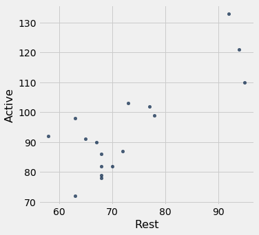
Here is a summary of the regression of the active pulse rate on the resting pulse rate for these data. Since the population consists just of male smokers, the parameters in the model might have different values from those in the previous exercise.
| Dep. Variable: | Active | R-squared: | 0.645 |
|---|---|---|---|
| Model: | OLS | Adj. R-squared: | 0.622 |
| Method: | Least Squares | F-statistic: | 27.29 |
| Date: | Sat, 07 Dec 2019 | Prob (F-statistic): | 0.000103 |
| Time: | 12:25:30 | Log-Likelihood: | -61.906 |
| No. Observations: | 17 | AIC: | 127.8 |
| Df Residuals: | 15 | BIC: | 129.5 |
| Df Model: | 1 | ||
| Covariance Type: | nonrobust |
| coef | std err | t | P>|t| | [0.025 | 0.975] | |
|---|---|---|---|---|---|---|
| const | 9.9360 | 16.345 | 0.608 | 0.552 | -24.903 | 44.775 |
| Rest | 1.1591 | 0.222 | 5.224 | 0.000 | 0.686 | 1.632 |
| Omnibus: | 2.279 | Durbin-Watson: | 1.114 |
|---|---|---|---|
| Prob(Omnibus): | 0.320 | Jarque-Bera (JB): | 1.423 |
| Skew: | 0.456 | Prob(JB): | 0.491 |
| Kurtosis: | 1.915 | Cond. No. | 505. |
Warnings:
[1] Standard Errors assume that the covariance matrix of the errors is correctly specified.
a) Find the correlation between the active and resting pulse rates for these data and compare it with the corresponding value for all students.
b) Show the calculation that leads to the displayed confidence interval for the true slope of Rest.
c) Use the displayed confidence interval for the true intercept to provide the conclusion of a test of hypotheses \(H_0\): \(\beta_0 = 0\) versus \(H_A\): \(\beta_0 \ne 0\) at the 5% level. Explain your reasoning.
d) Show the calculation that leads to the displayed value of P>|t| for the intercept. Is the value consistent with your answer to Part c?
e) Use the displayed results for the slope of Rest to provide the conclusion of a test of hypotheses \(H_0\): \(\beta_1 = 0\) versus \(H_A\): \(\beta_1 \ne 0\) at the 1% level. Explain your reasoning.