12.3. Towards Multiple Regression#
This section is an extended example of applications of the methods we have derived for regression. We will start with simple regression, which we understand well, and will then indicate how some of the results can be extended when there is more than one predictor variable.
The data are from a study on the treatment of Hodgkin’s disease, a type of cancer that can affect young people. The good news is that treatments for this cancer have high success rates. The bad news is that the treatments can be rather strong combinations of chemotherapy and radiation, and thus have serious side effects. A goal of the study was to identify combinations of treatments with reduced side effects.
The table hodgkins contains data on a random sample of patients. Each row corresponds to a patient. The columns contain the patient’s height in centimeters, the amount of radiation, the amount of medication used in chemotherapy, and measurements on the health of the patient’s lungs.
hodgkins
| height | rad | chemo | base | month15 | difference |
|---|---|---|---|---|---|
| 164 | 679 | 180 | 160.57 | 87.77 | -72.8 |
| 168 | 311 | 180 | 98.24 | 67.62 | -30.62 |
| 173 | 388 | 239 | 129.04 | 133.33 | 4.29 |
| 157 | 370 | 168 | 85.41 | 81.28 | -4.13 |
| 160 | 468 | 151 | 67.94 | 79.26 | 11.32 |
| 170 | 341 | 96 | 150.51 | 80.97 | -69.54 |
| 163 | 453 | 134 | 129.88 | 69.24 | -60.64 |
| 175 | 529 | 264 | 87.45 | 56.48 | -30.97 |
| 185 | 392 | 240 | 149.84 | 106.99 | -42.85 |
| 178 | 479 | 216 | 92.24 | 73.43 | -18.81 |
... (12 rows omitted)
n = hodgkins.num_rows
n
22
The radiation was directed towards each patient’s chest area or “mantle”, to destroy cancer cells in the lymph nodes near that area. Since this could adversely affect the patients’ lungs, the researchers measured the health of the patients’ lungs both before and after treatment. Each patient received a score, with larger scores corresponding to more healthy lungs.
The table records the baseline scores and also the scores 15 months after treatment. The change in score (15 month score minus baseline score) is in the final column. Notice the negative differences: 15 months after treatment, many patients’ lungs weren’t doing as well as before the treatment.
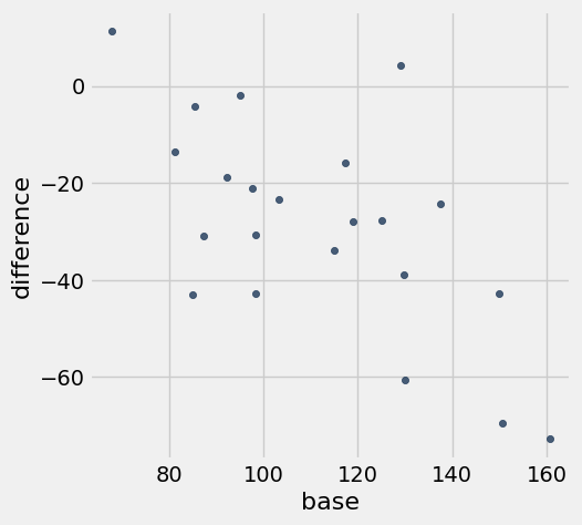
Perhaps not surprisingly, patients with larger baseline scores had bigger drops in score.
hodgkins.scatter('base', 'difference')
We will regress the difference on the baseline score, this time using the Python module statsmodels that allows us to easily perform multiple regression as well. You don’t have to learn the code below (though it’s not hard). Just focus on understanding an interpreting the output.
As a first step, we must import the module.
import statsmodels.api as sm
---------------------------------------------------------------------------
ValueError                                Traceback (most recent call last)
Cell In[6], line 1
----> 1 import statsmodels.api as sm

File /opt/miniconda3/lib/python3.12/site-packages/statsmodels/api.py:125
    114 from .genmod import api as genmod
    115 from .genmod.api import (
    116     GEE,
    117     GLM,
   (...)
    123     families,
    124 )
--> 125 from .graphics import api as graphics
    126 from .graphics.gofplots import ProbPlot, qqline, qqplot, qqplot_2samples
    127 from .imputation.bayes_mi import MI, BayesGaussMI

File /opt/miniconda3/lib/python3.12/site-packages/statsmodels/graphics/api.py:9
      7 from .gofplots import qqplot
      8 from .plottools import rainbow
----> 9 from .regressionplots import (
     10     abline_plot,
     11     influence_plot,
     12     plot_ccpr,
     13     plot_ccpr_grid,
     14     plot_fit,
     15     plot_leverage_resid2,
     16     plot_partregress,
     17     plot_partregress_grid,
     18     plot_regress_exog,
     19 )
     21 __all__ = [
     22     "abline_plot",
     23     "beanplot",
   (...)
     42     "violinplot",
     43 ]

File /opt/miniconda3/lib/python3.12/site-packages/statsmodels/graphics/regressionplots.py:23
     21 from statsmodels.genmod.generalized_linear_model import GLM
     22 from statsmodels.graphics import utils
---> 23 from statsmodels.nonparametric.smoothers_lowess import lowess
     24 from statsmodels.regression.linear_model import GLS, OLS, WLS
     25 from statsmodels.sandbox.regression.predstd import wls_prediction_std

File /opt/miniconda3/lib/python3.12/site-packages/statsmodels/nonparametric/smoothers_lowess.py:11
      2 """Lowess - wrapper for cythonized extension
      3
      4 Author : Chris Jordan-Squire
   (...)
      7
      8 """
     10 import numpy as np
---> 11 from ._smoothers_lowess import lowess as _lowess
     13 def lowess(endog, exog, frac=2.0/3.0, it=3, delta=0.0, xvals=None, is_sorted=False,
     14            missing='drop', return_sorted=True):
     15     '''LOWESS (Locally Weighted Scatterplot Smoothing)
     16
     17     A lowess function that outs smoothed estimates of endog
   (...)
    135
    136     '''

File statsmodels/nonparametric/_smoothers_lowess.pyx:1, in init statsmodels.nonparametric._smoothers_lowess()

ValueError: numpy.dtype size changed, may indicate binary incompatibility. Expected 96 from C header, got 88 from PyObject
The Table method to_df allows us to convert the table hodgkins to a structure called a data frame that works more smoothly with statsmodels.
h_data = hodgkins.to_df()
h_data
| height | rad | chemo | base | month15 | difference | |
|---|---|---|---|---|---|---|
| 0 | 164 | 679 | 180 | 160.57 | 87.77 | -72.80 |
| 1 | 168 | 311 | 180 | 98.24 | 67.62 | -30.62 |
| 2 | 173 | 388 | 239 | 129.04 | 133.33 | 4.29 |
| 3 | 157 | 370 | 168 | 85.41 | 81.28 | -4.13 |
| 4 | 160 | 468 | 151 | 67.94 | 79.26 | 11.32 |
| 5 | 170 | 341 | 96 | 150.51 | 80.97 | -69.54 |
| 6 | 163 | 453 | 134 | 129.88 | 69.24 | -60.64 |
| 7 | 175 | 529 | 264 | 87.45 | 56.48 | -30.97 |
| 8 | 185 | 392 | 240 | 149.84 | 106.99 | -42.85 |
| 9 | 178 | 479 | 216 | 92.24 | 73.43 | -18.81 |
| 10 | 179 | 376 | 160 | 117.43 | 101.61 | -15.82 |
| 11 | 181 | 539 | 196 | 129.75 | 90.78 | -38.97 |
| 12 | 173 | 217 | 204 | 97.59 | 76.38 | -21.21 |
| 13 | 166 | 456 | 192 | 81.29 | 67.66 | -13.63 |
| 14 | 170 | 252 | 150 | 98.29 | 55.51 | -42.78 |
| 15 | 165 | 622 | 162 | 118.98 | 90.92 | -28.06 |
| 16 | 173 | 305 | 213 | 103.17 | 79.74 | -23.43 |
| 17 | 174 | 566 | 198 | 94.97 | 93.08 | -1.89 |
| 18 | 173 | 322 | 119 | 85.00 | 41.96 | -43.04 |
| 19 | 173 | 270 | 160 | 115.02 | 81.12 | -33.90 |
| 20 | 183 | 259 | 241 | 125.02 | 97.18 | -27.84 |
| 21 | 188 | 238 | 252 | 137.43 | 113.20 | -24.23 |
There are several variables we could use to predict the difference. The only one we wouldn’t use is the 15 month measurement, as that’s precisely what we won’t have for a new patient before the treatment is adminstered.
But which of the rest should we use? One way to choose is to look at the correlation matrix of all the variables.
h_data.corr()
| height | rad | chemo | base | month15 | difference | |
|---|---|---|---|---|---|---|
| height | 1.000000 | -0.305206 | 0.576825 | 0.354229 | 0.390527 | -0.043394 |
| rad | -0.305206 | 1.000000 | -0.003739 | 0.096432 | 0.040616 | -0.073453 |
| chemo | 0.576825 | -0.003739 | 1.000000 | 0.062187 | 0.445788 | 0.346310 |
| base | 0.354229 | 0.096432 | 0.062187 | 1.000000 | 0.561371 | -0.630183 |
| month15 | 0.390527 | 0.040616 | 0.445788 | 0.561371 | 1.000000 | 0.288794 |
| difference | -0.043394 | -0.073453 | 0.346310 | -0.630183 | 0.288794 | 1.000000 |
Each entry in this table is the correlation between the variable specified by the row label and the variable specified by the column label. That’s why all the diagonal entries are \(1\).
Look at the last column (or last row). This contains the correlation between difference and each of the other variables. The baseline measurement has the largest correlation. To run the regression of difference on base we must first extract the columns of data that we need and then use the appropriate statsmodels methods.
First, we create data frames corresponding to the response and the predictor variable. The methods are not the same as for Tables, but you will get a general sense of what they are doing.
y = h_data[['difference']]  # response
x = h_data[['base']]        # predictor

# specify that the model includes an intercept
x_with_int = sm.add_constant(x)
The name of the OLS method stands for Ordinary Least Squares, which is the kind of least squares that we have discussed. There are other more complicated kinds that you might encounter in more advanced classes.
There is a lot of output, some of which we will discuss and the rest of which we will leave to another class. For some reason the output includes the date and time of running the regression, right in the middle of the summary statistics.
simple_regression = sm.OLS(y, x_with_int).fit()
simple_regression.summary()
| Dep. Variable: | difference | R-squared: | 0.397 |
|---|---|---|---|
| Model: | OLS | Adj. R-squared: | 0.367 |
| Method: | Least Squares | F-statistic: | 13.17 |
| Date: | Fri, 06 Dec 2019 | Prob (F-statistic): | 0.00167 |
| Time: | 22:34:07 | Log-Likelihood: | -92.947 |
| No. Observations: | 22 | AIC: | 189.9 |
| Df Residuals: | 20 | BIC: | 192.1 |
| Df Model: | 1 | ||
| Covariance Type: | nonrobust |
| coef | std err | t | P>|t| | [0.025 | 0.975] | |
|---|---|---|---|---|---|---|
| const | 32.1721 | 17.151 | 1.876 | 0.075 | -3.604 | 67.949 |
| base | -0.5447 | 0.150 | -3.630 | 0.002 | -0.858 | -0.232 |
| Omnibus: | 1.133 | Durbin-Watson: | 1.774 |
|---|---|---|---|
| Prob(Omnibus): | 0.568 | Jarque-Bera (JB): | 0.484 |
| Skew: | 0.362 | Prob(JB): | 0.785 |
| Kurtosis: | 3.069 | Cond. No. | 530. |
Warnings:
[1] Standard Errors assume that the covariance matrix of the errors is correctly specified.
There are three blocks of output. We will focus only on the the middle block.
constandbaserefer to the intercept and baseline measurement.coefstands for the estimated coefficients, which in our notation are \(\hat{\beta_0}\) and \(\hat{\beta_1}\).tis the \(t\)-statistic for testing whether or not the coefficient is 0. Based on our model, its degrees of freedom are \(n-2 = 20\); you’ll find this underDf Residualsin the top block.P > |t|is the total area in the two tails of the \(t\) distribution with \(n-2\) degrees of freedom.[0.025 0.975]are the ends of a 95% confidence interval for the parameter.
For the test of whether or not the true slope of the baseline measurement is \(0\), the observed test statistic is
The area in one tail is the chance that the \(t\) distribution with \(20\) degrees of freedom is less than \(-3.63\). That’s the cdf of the distribution evaluated at \(-3.63\):
one_tail = stats.t.cdf(-3.63, 20)
one_tail
0.0008339581409629714
Our test is two-sided (large values of \(\vert t \vert\) favor the alternative), so the \(p\)-value of the test is the total area of two tails, which is the displayed value \(0.002\) after rounding.
p = 2*one_tail
p
0.0016679162819259429
To find a 95% confidence interval for the true slope, we have to replace \(2\) in the expression \(\hat{\beta}_1 \pm 2SE(\hat{\beta}_1)\) by the corresponding value from the \(t\) distribution with 20 degrees of freedom. That’s not very far from \(2\):
t_95 = stats.t.ppf(0.975, 20)
t_95
2.0859634472658364
A 95% confidence interval for the true slope is given by \(\hat{\beta}_1 \pm t_{95}SE(\hat{\beta}_1)\). The observed interval is therefore given by the calculation below, which results in the same values as in the output of sm.OLS above.
# 95% confidence interval for the true slope

-0.5447 - t_95*0.150, -0.5447 + t_95*0.150
(-0.8575945170898753, -0.23180548291012454)
12.3.1. Multiple Regression#
What if we wanted to regress difference on both base and chemo? The first thing to do would be to check the correlation matrix again:
h_data.corr()
| height | rad | chemo | base | month15 | difference | |
|---|---|---|---|---|---|---|
| height | 1.000000 | -0.305206 | 0.576825 | 0.354229 | 0.390527 | -0.043394 |
| rad | -0.305206 | 1.000000 | -0.003739 | 0.096432 | 0.040616 | -0.073453 |
| chemo | 0.576825 | -0.003739 | 1.000000 | 0.062187 | 0.445788 | 0.346310 |
| base | 0.354229 | 0.096432 | 0.062187 | 1.000000 | 0.561371 | -0.630183 |
| month15 | 0.390527 | 0.040616 | 0.445788 | 0.561371 | 1.000000 | 0.288794 |
| difference | -0.043394 | -0.073453 | 0.346310 | -0.630183 | 0.288794 | 1.000000 |
What you are looking for is not just that chemo is the next most highly correlated with difference after base. More importantly, you are looking to see how strongly the two predictor variables base and chemo are linearly related to each other. That is, you are trying to figure out whether the two variables pick up genuinely different dimensions of the data.
The correlation matrix shows that the correlation between base and chemo is only about \(0.06\). The two predictors are not close to being linear functions of each other. So let’s run the regression.
The code is exactly the same as before, except that we have included a second predictor variable.
y = h_data[['difference']]      # response
x2 = h_data[['base', 'chemo']]  # predictors

# specify that the model includes an intercept
x2_with_int = sm.add_constant(x2)

multiple_regression = sm.OLS(y, x2_with_int).fit()
multiple_regression.summary()
| Dep. Variable: | difference | R-squared: | 0.546 |
|---|---|---|---|
| Model: | OLS | Adj. R-squared: | 0.499 |
| Method: | Least Squares | F-statistic: | 11.44 |
| Date: | Fri, 06 Dec 2019 | Prob (F-statistic): | 0.000548 |
| Time: | 22:34:31 | Log-Likelihood: | -89.820 |
| No. Observations: | 22 | AIC: | 185.6 |
| Df Residuals: | 19 | BIC: | 188.9 |
| Df Model: | 2 | ||
| Covariance Type: | nonrobust |
| coef | std err | t | P>|t| | [0.025 | 0.975] | |
|---|---|---|---|---|---|---|
| const | -0.9992 | 20.227 | -0.049 | 0.961 | -43.335 | 41.336 |
| base | -0.5655 | 0.134 | -4.226 | 0.000 | -0.846 | -0.285 |
| chemo | 0.1898 | 0.076 | 2.500 | 0.022 | 0.031 | 0.349 |
| Omnibus: | 0.853 | Durbin-Watson: | 1.781 |
|---|---|---|---|
| Prob(Omnibus): | 0.653 | Jarque-Bera (JB): | 0.368 |
| Skew: | 0.317 | Prob(JB): | 0.832 |
| Kurtosis: | 2.987 | Cond. No. | 1.36e+03 |
Warnings:
[1] Standard Errors assume that the covariance matrix of the errors is correctly specified.
[2] The condition number is large, 1.36e+03. This might indicate that there are
strong multicollinearity or other numerical problems.
Ignore the scary warning above. There isn’t strong multicollinearity (predictor variables being highly correlated with each other) nor other serious issues.
Just focus on the middle block of the output. It’s just like the middle block of the simple regression output, with one more line corresponding to chemo.
All of the values in the block are interpreted in the same way as before. The only change is in the degrees of freedom: because you are estimating one more parameter, the degrees of freedom have dropped by \(1\), and are thus \(19\) instead of \(20\).
For example, the 95% confidence interval for the slope of chemo is calculated as follows.
t_95_df19 = stats.t.ppf(0.975, 19)

0.1898 - t_95_df19*0.076, 0.1898 + t_95_df19*0.076
(0.03073017186497201, 0.348869828135028)
Finally, take a look at the value of R-squared in the very top line. It is \(0.546\) compared to \(0.397\) for the simple regression. It’s a math fact that the more predictor variables you use, the higher the R-squared value will be. This tempts people into using lots of predictors, whether or not the resulting model is comprehensible.
With an “everything as well as the kitchen sink” approach to selecting predictor variables, a researcher might be inclined to use all the possible predictors.
y = h_data[['difference']]      # response
x3 = h_data[['base', 'chemo', 'rad', 'height']]  # predictors

# specify that the model includes an intercept
x3_with_int = sm.add_constant(x3)

bad_regression = sm.OLS(y, x3_with_int).fit()
bad_regression.summary()
| Dep. Variable: | difference | R-squared: | 0.550 |
|---|---|---|---|
| Model: | OLS | Adj. R-squared: | 0.444 |
| Method: | Least Squares | F-statistic: | 5.185 |
| Date: | Fri, 06 Dec 2019 | Prob (F-statistic): | 0.00645 |
| Time: | 22:50:02 | Log-Likelihood: | -89.741 |
| No. Observations: | 22 | AIC: | 189.5 |
| Df Residuals: | 17 | BIC: | 194.9 |
| Df Model: | 4 | ||
| Covariance Type: | nonrobust |
| coef | std err | t | P>|t| | [0.025 | 0.975] | |
|---|---|---|---|---|---|---|
| const | 33.5226 | 101.061 | 0.332 | 0.744 | -179.698 | 246.743 |
| base | -0.5393 | 0.160 | -3.378 | 0.004 | -0.876 | -0.202 |
| chemo | 0.2124 | 0.103 | 2.053 | 0.056 | -0.006 | 0.431 |
| rad | -0.0062 | 0.031 | -0.203 | 0.841 | -0.071 | 0.059 |
| height | -0.2274 | 0.658 | -0.346 | 0.734 | -1.615 | 1.160 |
| Omnibus: | 0.589 | Durbin-Watson: | 1.812 |
|---|---|---|---|
| Prob(Omnibus): | 0.745 | Jarque-Bera (JB): | 0.321 |
| Skew: | 0.286 | Prob(JB): | 0.852 |
| Kurtosis: | 2.851 | Cond. No. | 1.46e+04 |
Warnings:
[1] Standard Errors assume that the covariance matrix of the errors is correctly specified.
[2] The condition number is large, 1.46e+04. This might indicate that there are
strong multicollinearity or other numerical problems.
This is not a good idea. We end up with a far more complicated model for no appreciable gain in R-squared. The “adjusted \(R^2\)” penalizes us for using more predictor variables: notice that the value of Adj. R-squared is smaller for the regression with all the predictors than for the regression with just base and chemo.
Curious about how to select predictors, or about what makes a good regression? Then take some more statistics classes! This one is complete.