2.4. Use and Interpretation#
There are many situations in the law, medicine, and other fields, where Bayes’ Rule might help make decisions.
Given the evidence, is the defendant guilty or not?
Given the test results, does the patient have the disease, or not?
But not all medical or legal professionals have taken data science classes. So the calculations are sometimes misinterpreted or done incorrectly or simply not done at all.
Here is an example that demonstrates some of the issues that are involved.
2.4.1. Harvard Medical School Survey#
In 1978, Cascella, Schoenberger, and Grayboys asked 60 physicians, students, and house officers at the Harvard Medical school the following question:
“If a test to detect a disease whose prevalence is 1/1,000 has a false positive rate of 5 per cent, what is the chance that a person found to have a positive result actually has the disease, assuming that you know nothing about the person’s symptoms or signs?”
The answers ranged from about 2% to 95%, with 27 out of the 60 Medical School members surveyed answering 95%.
Let’s see what we think the answer should be. First, some background and terminology:
Prevalence in the population is the percent of people who have the disease. It is also called the base rate of the disease.
There is a test for the disease that has two possible results for a tested person. A positive result means that according to the test the person has the disease. A negative result means that according to the test the person doesn’t have the disease.
The test can give a wrong result. The false positive rate is the proportion of positive results among people who don’t have the disease.
The true positive rate is the rate of positive results among those who do have the disease. The question doesn’t provide this rate. We will assume, as the people surveyed also did, that the test is good and the true positive rate is 100%.
Here are the data in a tree diagram.
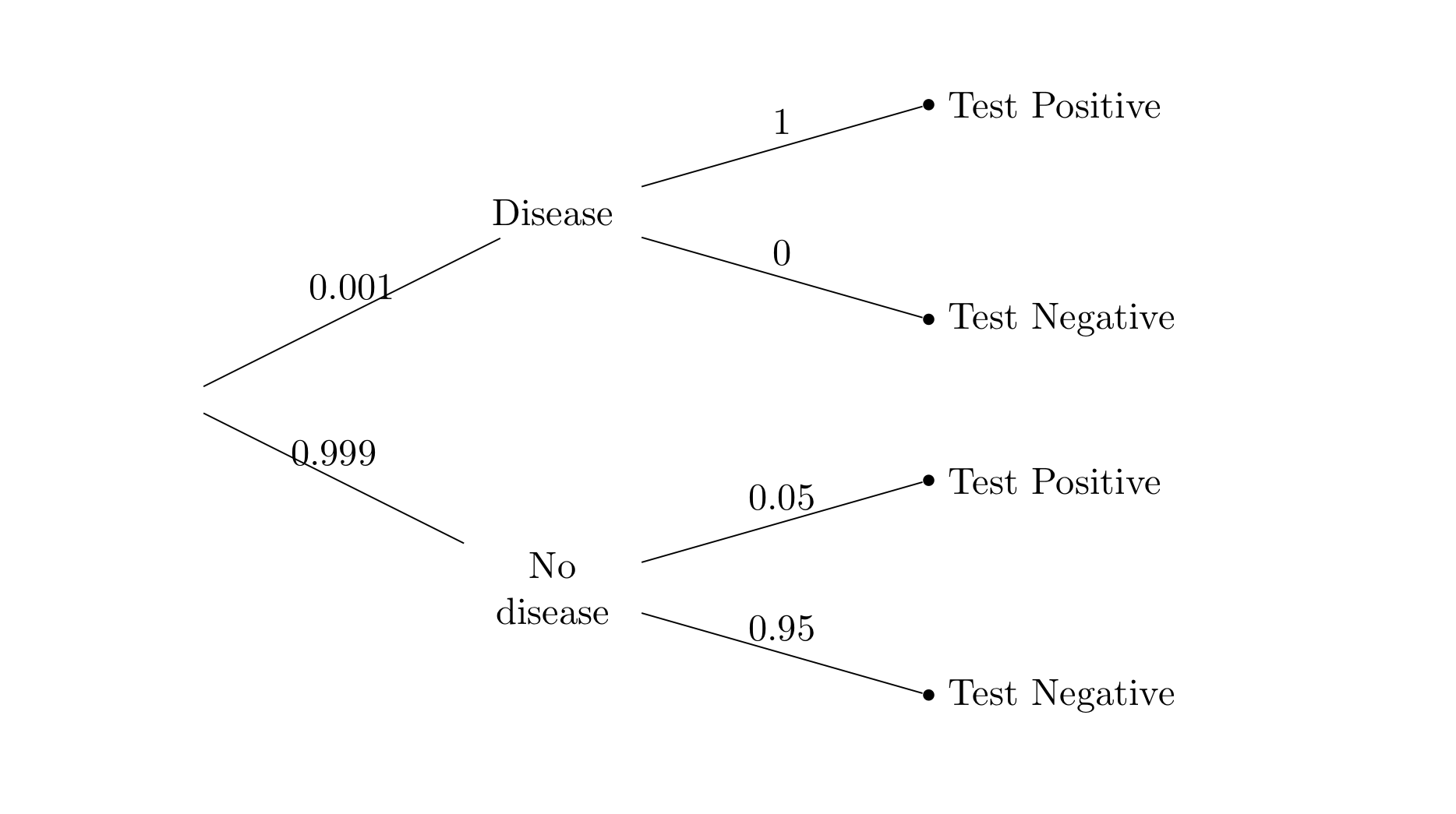
The question asks for a chance but doesn’t say how the person is selected. As a first step, let’s assume that the person was selected at random from the population. Then the answer is a straightforward application of Bayes’ Rule:
This calculation explains the answer of approximately 2% that was provided by 11 out of the 60 people surveyed.
2.4.2. Prior and Posterior Rates#
While the answer above is numerically correct, it is rather unsettling.
The medical test is pretty accurate. For a person who has the disease the test is error-free – it will always make the correct conclusion. For a person who doesn’t have the disease the test has an error rate of only 5%. For these people it will make the correct conclusion 95% of the time.
Yet for a randomly selected person who has tested positive, the calculation says the chance of disease is a mere 2%.
To understand what the 2% means, remember that it is a posterior probability of disease: the probability that the person has the disease, given that they tested positive.
This should be compared to the prior probability of disease: the probability we assigned to the person having the disease before we knew anything about test results. That probability was the base rate of 0.001, which is 0.1%.
Knowing that the person tested positive increased this probability by a factor of 20.
2.4.3. Effect of a Low Base Rate#
If 2% still seems small as an answer, look at the table below. It pretends that the population consists of 100,000 people, and displays the counts in the four branches of the tree. You can redo the table with a different population size if you wish, as long as you keep the proportions consistent with the question.
Test Positive |
Test Negative |
|
|---|---|---|
Disease |
100 |
0 |
No Disease |
4,995 |
94,905 |
As described in the question, 100 out of the 100,000 people (1/1000) have the disease. All these people test positive. Of the 99,900 people who don’t have the disease, 4,995 (5%) falsely test positive and the rest test negative.
If a randomly picked person has the disease, they are one of the people in the Test Positive column. This column illuminates an aspect of the calculation that must be understood in order to correctly interpret the result.
There are two groups of people who test positive: all those who have the disease, and also 5% of those who don’t have the disease.
The base rate is very small: the disease is rare in the population. So even though everybody with the disease tests positive, their number is small (100) in comparison to the group of people who don’t have the disease and falsely test positive (4,995). So the people who correctly test positive are a small fraction of all the people who test positive.
That is why when we are given that the test result of a randomly chosen person is positive, we conclude that there is a small chance that the person has the disease.
2.4.4. Base Rate Fallacy#
How could 27 out of the 60 Medical School members surveyed end up with an answer of 95% instead? It is because they made a common mistake known as the base rate fallacy. This error consists of simply ignoring the base rate and just focusing on the likelihoods.
Since the test had a 5% false positive rate, 27 people ignored all else and answered 95%, not noticing that they had provided \(P(\text{test negative} \mid \text{no disease})\) when instead the question asked for \(P(\text{disease} \mid \text{test positive})\).
The authors of the survey scathingly concluded that, “… formal decision analysis was almost entirely unknown and even common-sense reasoning about the interpretation of laboratory data was uncommon.”
Ouch. But the Med School members have plenty of company. The base rate fallacy occurs with depressing frequency in medicine, the law, and other fields. For some people who are not trained in data science, it is hard to keep track of several different rates at once and combine them appropriately.
2.4.5. Changing the Base Rate#
The most unsettling aspect of the Bayes’ Rule calculation above is the prior probability of 0.001. It is based on the assumption that the person was picked randomly from the population. But medical tests aren’t given to random members of the public. People get tested when they or their doctors think they might be at risk for the disease. In that case the base rate might not be the right figure to use for the prior probability of disease.
Suppose instead a person thinks that there is a small chance, say 10%, that they have the disease. If this person’s test result comes out positive, how should they update their probability of disease?
Since the test remains the same, all that has to change in the tree diagram is the prior probability of having and not having the disease.
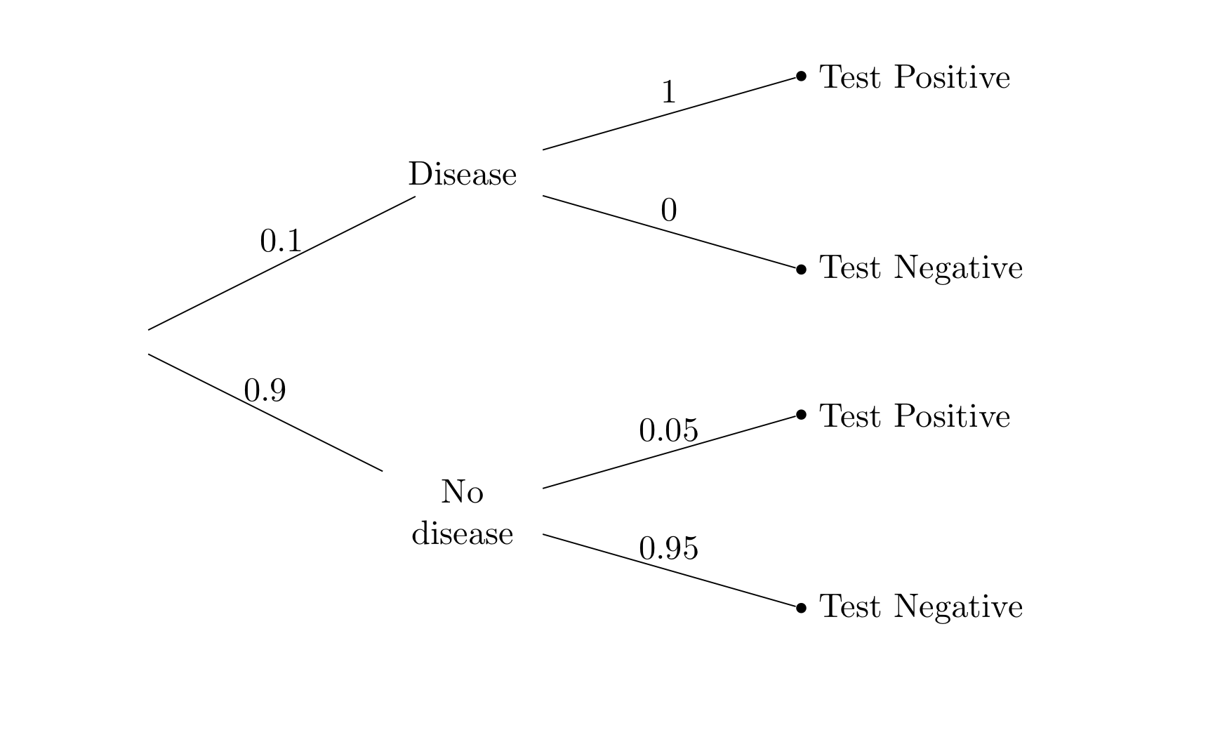
The calculation changes to
The change in the prior probability of disease from 0.1% to 10% has a massive effect on the posterior probability of disease given a positive test result. That is now close to 70%.
The main lesson is that posterior probabilities are affected by the base rate as well as the likelihoods. Ignoring either of these can result in errors of calculation and interpretation.