4.1. Cumulative Distribution Function (CDF)

There are many ways of specifying distributions. We have sometimes used a table to display the distribution of a random variable \(X\). At other times we have written \(P(X = k)\) as a formula for each possible value \(k\) of \(X\).

Another useful function that encapsulates all the information about the distribution of \(X\) is called the cumulative distribution function of \(X\). That’s a real mouthful, so it is usually abbreviated to the cdf of \(X\).

Let’s see what the cdf is in an example.

Suppose \(X\) has the distribution given below. It happens to be the binomial \((3, 1/2)\) distribution, but that is not important for this discussion.

\(~~~~~~~~~~~~~~~~~~~~~x\)	0	1	2	3
\(P(X=x)\)	1/8	3/8	3/8	1/8

The cdf of \(X\) is another way of providing the same information. It is the function \(F\) defined by

\[ F(x) ~ = ~ P(X \le x), ~~~~~ -\infty < x < \infty \]

The cdf of the random variable \(X\), evaluated at the point \(x\), is the chance that the value of \(X\) is at most \(x\).

The gold area in the probability histogram below is \(F(2)\).

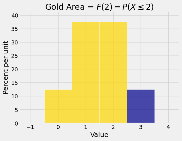
We will sometimes use the loose term “left hand probabilities” to denote values of \(F\). Each of those values \(F(x)\) is the area of the bar at \(x\) as well as all the bars to the left. In the figure above,

\[ F(2) ~ = ~ P(X \le 2) ~ = ~ P(X = 0) + P(X = 1) + P(X = 2) \]

We will now augment the distribution table by a row containing some values of \(F\). These are obtained obtained by adding the probabilities \(P(X=x)\) successively from the left end. This cumulative sum is the reason for the name of the function.

\(~~~~~~~~~~~~~~~~~~~~~x\)	0	1	2	3
\(P(X=x)\)	1/8	3/8	3/8	1/8
\(F(x)\)	1/8	4/8	7/8	1

Notice that we can recover \(P(X=x)\) from values of \(F\) as follows. For integer \(x\),

\[ P(X = x) ~ = ~ P(X \le x) - P(X \le x-1) ~ = ~ F(x) - F(x-1) \]

These calculations show that if you know the distribution of \(X\) then you know the cdf of \(X\), and vice versa. The distribution and the cdf contain the same information.

4.1.1. Graph of the CDF

The graph of every cdf has some properties that are easy to see:

• The graph is non-decreasing.

• The values are on the vertical axis are probabilities and hence are between 0 and 1.

• The graph starts out at or near 0 for large negative values of \(x\), and ends up at or near 1 for large positive values of \(x\).

You can see all these properties in the graph of the function \(F\) defined above.

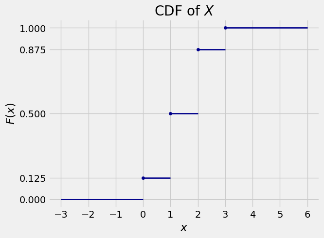
You can see also that the graph has flat parts and jumps.

• Flat parts: These are in-between the possible values of \(X\) and also beyond the possible values in both directions. Since \(X\) is a non-negative variable, for all negative \(x\) we have \(F(x) = P(X \le x) = 0\). Since \(X\) is always at most 3, for all \(x > 3\) we have \(F(x) = P(X \le x) = 1\). For \(x\) in between two possible values, say \(x = 1.6\), we have \(F(1.6) = P(X \le 1.6) = P(X \le 1) = F(1)\). So for \(x \in [1, 2)\), the graph is flat at \(F(1)\). You can explain all the other flat parts analogously.

• Jumps: The graph has a jump (or discontinuity) at each possible value \(x\) of \(X\). That is, the graph jumps at each value \(x\) such that \(P(X = x) > 0\). The size of the jump at \(x\) is equal to \(P(X = x)\). For example, \(P(X = 2)\) is the size of the jump at \(x=2\), which is \(0.875 - 0.5 = 0.375 = 3/8\).

4.1.2. Computation

We will have many uses for the cdf in this course. In fact, we have already used it several times without giving it a name.

For example, the chance of at most 3 sixes in 20 rolls of a die is given by the binomial formula and the addition rule:

\[ P(\text{at most 3 sixes in 20 rolls}) ~ = ~ \sum_{k=0}^3 \binom{20}{k}(1/6)^k(5/6)^{20-k} \]

This can be computed as

sum(stats.binom.pmf(np.arange(4), 20, 1/6))

0.5665456377756696

Let \(X\) be the number of sixes in 20 rolls. Then \(X\) has the binomial \((20, 1/6)\) distribution. The answer above is \(P(X \le 3)\). That’s \(F(3)\) where \(F\) is the cdf of \(X\).

The stats module includes a cdf method that allows us to obtain the answer directly without summing.

The expression stats.binom.cdf(k, n, p) evaluates to \(F(k)\) where \(F\) is the cdf of a binomial \((n, p)\) random variable.

So our answer can also be found as follows.

stats.binom.cdf(3, 20, 1/6)

0.566545637775669

Probabilities are frequently computed as sums. The cdf is a very useful tool for doing this, so stats provides a cdf method associated with each distribution.

You can use stats.hypergeom.cdf(k, N, G, n) to find the value of \(F(k)\) for a random variable that has the hypergeometric \((N, G, n)\) distribution.

For example, recall that a standard deck contains 52 cards of which 12 are face cards. The chance of more than 5 face cards in a bridge hand of 13 cards dealt from a standard deck is

\[\begin{split} \begin{align*} &P(\text{more than 5 face cards in a hand of 13 cards}) \\ &= ~ 1 - P(\text{at most 5 face cards in the hand}) \\ &= ~ 1 - \sum_{k=0}^{5} \frac{\binom{12}{k}\binom{40}{13-k}}{\binom{52}{13}} \end{align*} \end{split}\]

Now you can get the numerical value by using stats.hypergeom.cdf:

1 - stats.hypergeom.cdf(5, 52, 12, 13)

0.03246092516982357