11.1. Bias and Variance

Suppose we are trying to estimate a constant numerical parameter \(\theta\), and our estimator is the statistic \(T\). Remember that a statistic is a number that we can calculate from our random sample; since the sample is random, so is the statistic.

To assess the quality of an estimator, we have to examine how its values compare with the parameter being estimated. We will first do a qualitative analysis and then move on to formal definitions.

Each figure below corresponds to a different estimator. In each case, the parameter \(\theta\) is at the red dot on the number line. We have generated a few values of the estimator and have plotted them in blue.

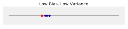• The figure on the top left corresponds to an estimator that is unbiased and has low variance. Its values are tightly clustered around the red dot. This kind of estimator is desirable: it is rarely far from the parameter, and it doesn’t systematically overestimate or underestimate.

• The figure on the bottom left corresponds to an estimator that has low variance but is biased. We will give a formal definition of bias later in this section; for now, just think of bias as a systematic overestimation or underestimation. The estimator in this figure overestimates by quite a bit compared to the estimators in the other figures.

• The figure on the top right corresponds to an estimator that is unbiased but has high variance. The six values plotted do look roughly evenly distributed around the red dot, but some of them are quite far from the red dot, on either side.

• The figure on the bottom right corresponds to an estimator that has low variance and also low bias. It’s not unbiased – you can see that it overestimates in general. But not by much! And because of its low variance, it is rarely very far from the parameter. So, even though the estimator is biased, we might want to use it because we know its value will be close to the parameter.

Now let’s attempt a quantitative analysis of what we have seen.

11.1.1. Mean Squared Error

The error in our estimate is \(T - \theta\). The mean squared error of the estimator \(T\) is defined as

\[ MSE_\theta(T) ~ = ~ E_\theta\left((T - \theta)^2\right) \]

We are using \(\theta\) as a subscript to remind us that the expectation is calculated under the assumption that \(\theta\) is the true value of the parameter.

The mean squared error can be used to assess the quality of an estimator: lower is better.

11.1.2. Decomposition of Error

Let’s try and understand the reasons why there is error in our estimate.

The first reason is that values of \(T\) depend on the sample and can therefore vary. The expected value is \(E_\theta(T)\), but \(T\) will typically differ from that. The difference is the familiar deviation

\[ D_\theta(T) ~ = ~ T - E_\theta(T) \]

The deviation \(D_\theta(T)\) is a random variable.

The second reason for the error is bias, which we will now define formally.

Recall that in an earlier chapter we defined \(T\) to be an unbiased estimator of \(\theta\) if \(E_\theta(T) = \theta\). But estimators can be biased. The bias of the estimator \(T\) is defined to be the amount by which its expectation exceeds the parameter:

\[ B_\theta(T) ~ = ~ E_\theta(T) - \theta \]

Both \(E_\theta(T)\) and \(\theta\) are constants, so the bias \(B_\theta(T)\) is a constant. It’s not a random variable.

If the bias is positive, then \(T\) tends to overestimate \(\theta\). If the bias is negative, then \(T\) tends to underestimate \(\theta\).

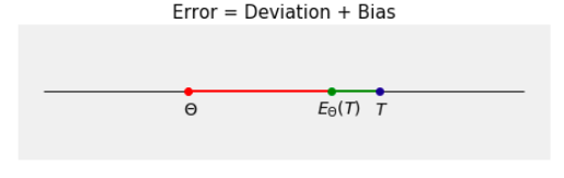
We now have a decomposition of the error as the sum of the deviation and the bias:

\[\begin{split} \begin{align*} T - \theta ~ &= ~ \big{(}T - E_\theta(T)\big{)} + \big{(} E_\theta(T) - \theta \big{)} \\ &= ~ D_\theta(T) + B_\theta(T) \end{align*} \end{split}\]

The figure below illustrates the decomposition. The green segment represents the deviation and the red segment is the bias.

11.1.3. Bias-Variance Decomposition

This leads to a decomposition of the mean squared error.

\[\begin{split} \begin{align*} MSE_\theta (T) ~ &= ~ E_\theta \left( (T - \theta)^2 \right) \\ &= ~ E_\theta \left( (D_\theta(T) + B_\theta(T))^2 \right) \\ &= ~ E_\theta \left( D_\theta^2(T) + 2D_\theta(T)B_\theta(T) + B_\theta^2(T) \right) \\ &= ~ E_\theta(D_\theta^2(T)) + 2B_\theta(T)E_\theta(D_\theta(T)) + B_\theta^2(T) \\ &= ~ Var_\theta(T) + B_\theta^2(T) \end{align*} \end{split}\]

The last line follows from two facts about the deviation \(D_\theta(T)\):

• Deviations average out to zero: \(E_\theta(D_\theta(T)) = 0\).

• By the definition of variance, \(Var_\theta(T) = E_\theta(D_\theta^2(T))\)

The bias-variance decomposition says

\[ \text{mean squared error} ~ = ~ \text{variance} + \text{bias}^2 \]

This quantifies what we saw visually: the quality of an estimator depends on the bias as well as the variance.

Ideally, we would like to construct an estimator for which both the bias and the variance are small. Sometimes this turns out to be impossible. For example, if you adjust an estimator to reduce bias, you might end up increasing the variance.

Notes

• The second term on the right hand side is the square of the bias, not just the bias. The bias has the same units of measurement as \(T\) and \(\theta\). The square of the bias is in the square of those units, like the mean squared error and the variance.

• It’s clear from the diagrams at the start of this section that variance and bias are important in assessing how good \(T\) is as an estimator. The bias-variance decomposition shows that there is no other aspect of \(T\) that contributes to the mean square error.

• The MSE, bias, and variance of \(T\) all depend on \(\theta\). We typically don’t know the parameter \(\theta\), so we can’t compute numerical values of these quantities. But we can work with them as functions of \(\theta\). For example, if one estimator has variance \(\theta^2\) and another estimator has variance \(2\theta^2\), then we know that the second one has the higher variance for every value of \(\theta\).